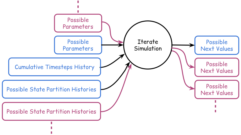
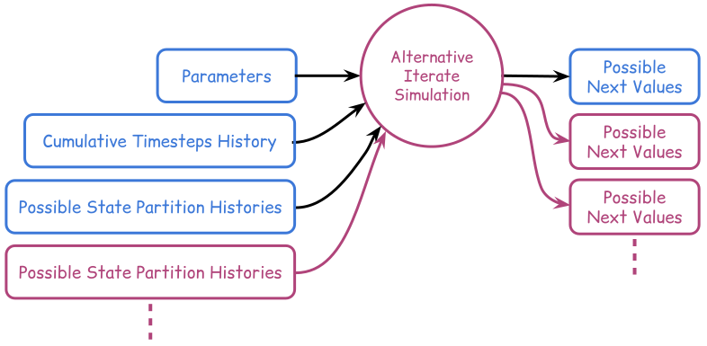
Preparing a simulation for action-taking

The two kinds of sensitivity

Data Scientists will often ask the following question about their models: if I change this input, how will my model prediction change?

Let’s give a name to this idea, and call it ‘prediction sensitivity’.

But the question we were asking at the end of the last post was more aligned with: if I change this input, how will my taken action change?

Let’s call this one ‘action-taking sensitivity’.

Both questions are referring to ‘inputs’ when this really means changing one of two things: changing logic/structure or changing parameters.

If we want to learn parameters which correspond to optimal simulation trajectories, we first need to specify what ‘optimal’ means.

We do this by defining an objective whose maximum/minimum possible value will be achieved when our goal is met.

For instance, we may define some logic in a state partition iteration of the simulation which replicates taking ‘actions’ in the real world. This logic can depend on the simulation parameters so that the latter encodes the behaviour quantitatively.

Given this setup, a very common goal of interest is then in finding the best actions to take; which is analogous to optimising the parameters of the action-taking state partition iteration. We will refer to these parameters as ‘policy parameters’.

But what should be use as an objective?

The ‘discounted future reward’ is a quantity we can specify that a simulation trajectory will have accumulated into the future, accounting for increasing distance into the future by ‘discounting’ it gradually with a weighting.

We are using this concept of discounted future reward in the same way that it is used in reinforcement learning.

The idea is that, as you go further into the future, the importance of the reward you have accumulated by then is increasingly irrelevant to actions you might take at the present moment.

Example: Optimising with evolutionary strategies

The evolutionary strategies algorithm can be applied to search future simulation trajectories to find the best set of policy parameters needed to achieve some discounted future reward.

This algorithm relies on sorting the sampled simulation trajectories according to their discounted future rewards and then using the top fraction of these to update the best known policy parameters (and the variance around them) after each timestep.

Which action-taking policy logic finds the best actions?

How sensitive is this choice to changes in the data? How sensitive is this choice to changes in the outcome model?

Answers to both of these questions tell us how the action-taking policy generalises within the problem domain to alternative scenarios and underlying system mechanisms.

How sensitive is this choice to changes in the action parameters?

In much the same way as it does in learning simulations of the real world answering this question tells us how sloppy the action-taking policy is, and as a result how generalisable it could be to other problem domains.

Explaining why the simulation predicts what it does

Cover these topics: - past-looking simulation graph analysis - forward-looking counterfactual analysis: simulation differencing and why SHAP is better - forward-looking counterfactual analysis: simulation SHAP analysis

Inferring which simulation to use

Cover these topics: - Bayesian model selection applied to action-taking is the same as doing causal inference