Learning simulations of the real world

What is our objective?

Unlike machine learning models, which typically come with standard training algorithms (like backpropagation for neural networks), simulations often need us to explicitly choose and design procedures for learning their parameters from real-world data or optimising their outputs.

In order to do this, we must first have some objective which either characterises how close simulation trajectories are to replicating the data we have or define the quantity we want to optimise.

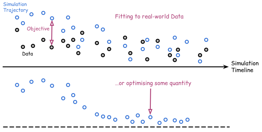
There are a number of techniques we can use to specify what the objective should be, depending on the purpose.

Learning parameters from data

If we want to learn the parameters which correspond to simulation trajectories fitting real-world data trends more closely, it is natural to use an objective based on the probabilities of state partition histories that we computed in the previous post.

We start by streaming time-series data into our simulation by specifying it as a state partition.

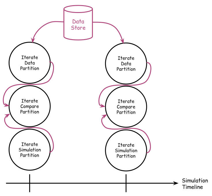
We can then use a method to estimate the probabilities of state values within the data, e.g., the probabilistic sample weighting we discussed in the previous post.

So we have a way to calculate these ‘data probabilities’ for any possible state values the data can take in time.

By then evaluating these data probabilities at the points which coincide with simulation trajectories, we have an objective which quantifies how close the simulation is to the data.

When talking about different values for this objective, we often use the terminology ‘quality of fit’ or ‘fit to the data’ to describe how close the simulation is to replicating the data, and hence how good the value of the objective is.

Example: Online simulation parameter estimation

The data probabilities of simulation trajectories can also be interpreted as probabilities of simulation parameters; often accompanied with some simulation noise to account for differences between trajectories even with the same parameters.

We can create an algorithm which uses this sequence of probabilities to estimate the probabilities of simulation parameters in a very similar way to probabilistic sample weighting (see the last post for details on the latter).

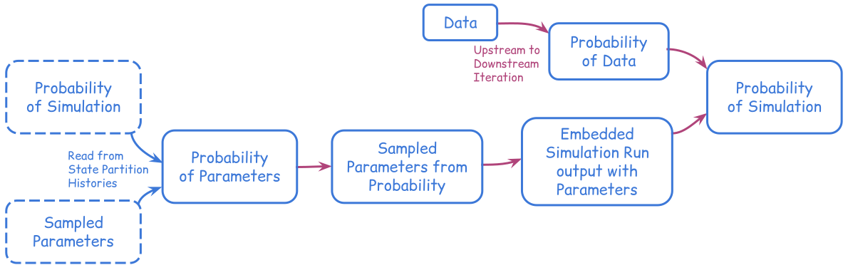
We might call this algorithm ‘online simulation parameter estimation’; where ‘online’ here means that the simulation is being adaptively learned to the data iteratively in time, as opposed to a whole batch all at once.

Simulation sloppiness isn’t bad

So we have a simulation which is able to learn its parameters from real world data.

How sensitive is the simulation-data fit to changes in the parameters? In other words, how sloppy is the simulation?

If a simulation is sloppy it means that it has many additional parameters which can be varied that do not strongly affect the quality of fit to the dataset of interest. We typically call this kind of parameter ‘unconstrained’ by the data.

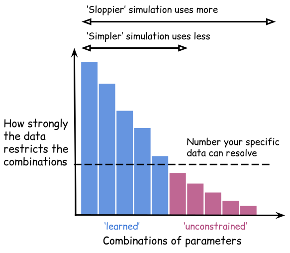
Simulation sloppiness sounds bad; but it has been shown that machine learning models with more sloppiness have a tendency to generalise better to new datasets.

Learning simulation structure from data

There is usually more than one simulation structure that can be a viable model for the real world system of interest, and these often have different numbers of parameters.

Choosing between different simulation structures should, in principle, be as easy as selecting the one with the best overall value for the objective. But it is actually more complicated than this because you can have complex or simple models which fit the data equally well.

Let’s say we have two different simulation structures which we are comparing by fitting them to the same dataset. Let’s also say that one of these simulations has lots of parameters and the other has much fewer.

We might interpret the concept of sloppiness to mean that the simulation which has more parameters is always the better choice. This would be wrong without a deeper analysis.

Remember that simulation sloppiness refers to parameters which are not constrained by the data.

What we need to find out is how many parameters are constrained (or learned) by the data in both simulations. In other words; how many parameters does each simulation have which the objective value is sensitive to changing?

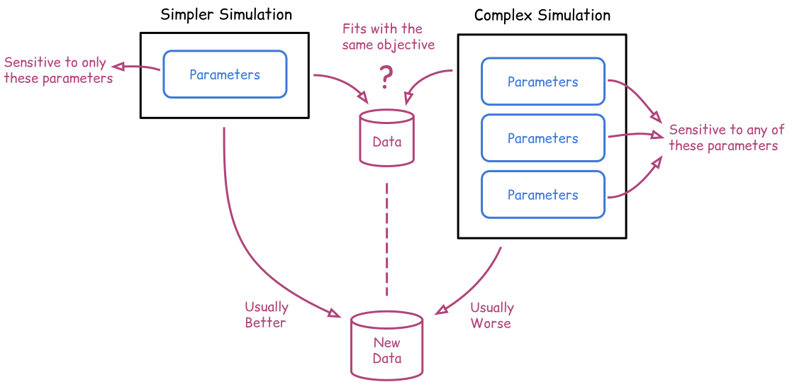
The general wisdom is to prefer simulations and models with fewer constrained parameters.

Why? Think about the parameter sensitivity of the quality of fit: if there are more parameters being constrained by the data, this means that the objective value is sensitive to more parameters. So there are more ‘moving parts’ to the simulation which have a greater chance of being misaligned with some new data we haven’t seen yet.

We can think of simulations with fewer constrained parameters (but equal quality of fit) to be more likely to generalise across different datasets from a systems of the same, or similar, type in the real world. This also indicates more fundamental mechanisms are being learned from the data that are potentially transferrable to other systems.

Example: Counting the parameters which are constrained

Let’s imagine two different simulation structures being fit to the same dataset. The simple structure has 3 parameters, while the complex one has 7.

Let’s also imagine that the complex structure always fits the observed data at least as well as the simple one; so the objective value on its own can never tell you which structure to choose.

Switching between the two structures, we can compare how many of their parameters the data actually constrains, and then use this as a way to choose between them.